BigQuery Graph Measures in Data Studio: Build a Data Source with Multi-Grain Aggregation

---

“What’s the average basket on my e-commerce site when there’s a promo item in the cart?”

A simple question from a merchandising team. On an item-grain reporting table, the promo flag lives on the item line, while the order revenue is repeated on every item line of the same order. Answering it in Data Studio means counting each order once, whatever the breakdown.

We all know the workarounds: one table per grain, a blend per chart, a custom query per question. These kinds of solutions work, but they also multiply the objects to maintain, and the next person who builds a chart on the same data source will fall into the same trap.

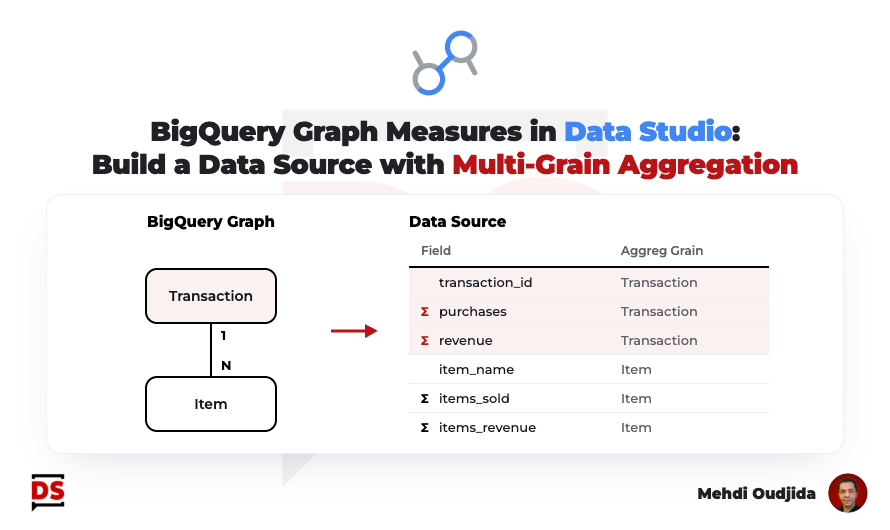
A few weeks ago, the Data Studio team released a rather discreet feature: Data Studio can now connect to a BigQuery Graph and import its measures as metrics. Behind it, there is a simple promise for anyone who prepares reporting tables in BigQuery: declare once, in BigQuery, at which grain each metric must be aggregated, and let every Data Studio chart respect it.

My example is based on GA4 e-commerce data but, as usual, the same approach applies to any reporting table mixing several grains.

In this article, you will discover how to build a multi-grain data source for your Data Studio reports, where BigQuery Graph measures keep each metric at the right grain, whatever the breakdown.

---

The result

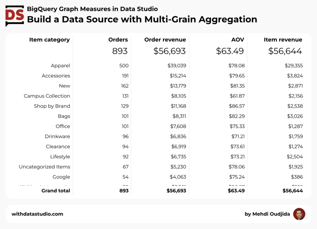
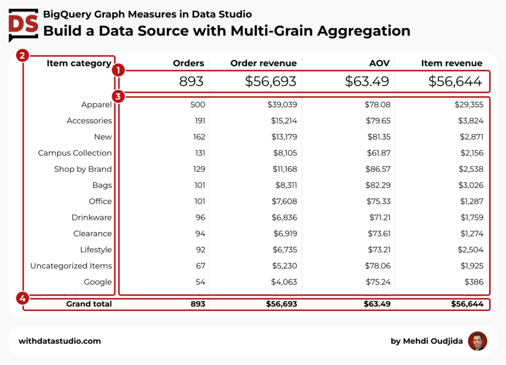
The Data Studio report page below displays statistics from a single data source, at two grains: orders and items. Its charts combine order metrics and item metrics, broken down by product category, and none of them counts an order twice.

---

What is BigQuery Graph, measures & aggregation grain

BigQuery Graph lets you model existing tables as a graph: nodes for your entities (orders, items, customers) and edges for the relationships between them (an item belongs to an order).

Three things matter for a reporting use:

• No data copy. A graph is defined on top of existing tables or views. It behaves like a logical view: queries read the tables as they are at execution time.
• A dataset object. You create it next to your tables and views, and it appears in the BigQuery Explorer.
• A semantic layer. Beyond the relationships, the graph can carry descriptions, synonyms and measures.

BigQuery Graph is known for path queries, like fraud detection or identity resolution. We won’t use any of that. For a Data Studio report creator, the interesting part is the measures.

A measure is an aggregated property declared on a node, for example the sum of the order revenue.

The key point: a measure is aggregated relative to the key of its node. Declared on an order node keyed by transaction_id, the order revenue is counted once per order, even when the query joins the items and duplicates the order rows. The usual fan-out disappears by construction.

Measures support SUM, AVG, COUNT, MIN and MAX, and can be combined into derived measures, like an average order value built from the revenue and the number of orders. Derived measures keep the same protection.

In BigQuery, a graph with measures is queried in SQL which applies each measure at its own grain.

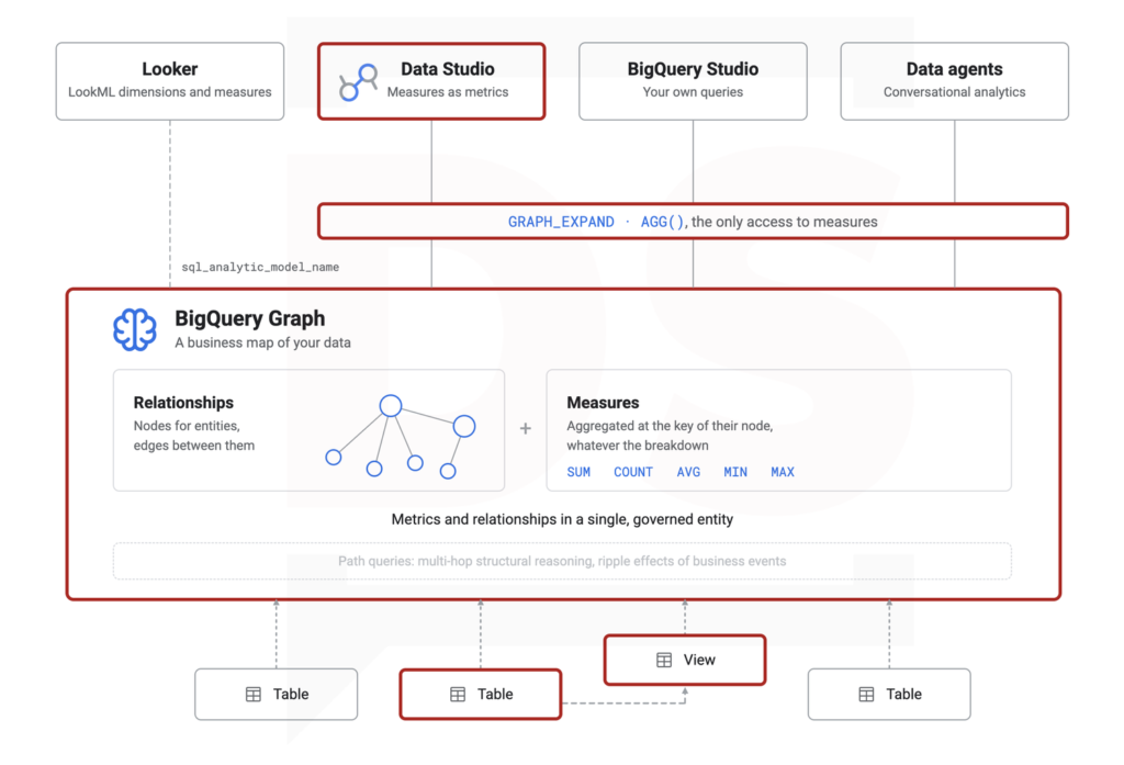
In Data Studio, you don’t even have to write that query. When you connect a data source to the graph, its measures become metrics whose aggregation type can’t be changed in the report. The aggregation rule lives in BigQuery, not in each chart.

---

Ingredients

For this configuration, we will need the following elements:

• An item-grain reporting table in BigQuery.
• A BigQuery property graph declaring the order and item measures.
• A Data Studio data source connected to the graph.
• Charts mixing order and item metrics.

On the BigQuery side, you need a project with on-demand pricing, or a reservation in the Enterprise or Enterprise Plus edition: graph measures aren’t available with the Standard edition. The BigQuery Data Editor role on the dataset is enough to create the view and the graph.

No graph query language here. Everything in this tutorial is plain SQL.

---

The BigQuery reporting table at the item grain

Let’s consider that your pipeline already provides a reporting table with one line per item sold, and the order fields repeated on each line.

For my example, I use viz_purchase_items, with purchases from a GA4 export. See the related schema below.

Field	Type	Grain
data_date	DATE	order
transaction_id	STRING	order
transaction_revenue	FLOAT64	order, repeated on each item line
item_index	INT64	item
item_id	STRING	item
item_category	STRING	item
item_name	STRING	item
item_sold_quantity	INT64	item
item_revenue	FLOAT64	item

Used as is in Data Studio, this kind of table makes it impossible to aggregate transaction_revenue correctly, once per order, because it is repeated on every item line. This is where BigQuery Graph measures come into play.

---

Property graph with order and item measures

Now, let’s create the graph with a single script, including a small view for the order grain.

View and property graph with measures

CREATE OR REPLACE VIEW `your-project.your_dataset.v_purchases` AS
SELECT
  transaction_id,
  ANY_VALUE(data_date) AS data_date,
  ANY_VALUE(transaction_revenue) AS raw_transaction_revenue
FROM `your-project.your_dataset.viz_purchase_items`
GROUP BY ALL;

CREATE OR REPLACE PROPERTY GRAPH `your-project.your_dataset.purchase_graph`
  NODE TABLES (
    `your-project.your_dataset.v_purchases` AS Purchase
      KEY (transaction_id)
      PROPERTIES (
        transaction_id,
        data_date,
        raw_transaction_revenue AS raw_transaction_revenue
          OPTIONS (description = "Order revenue as stored, one value per order. Use the transaction_revenue measure as a metric."),
        MEASURE(COUNT(transaction_id)) AS purchases
          OPTIONS (description = "Number of orders. Aggregated once per order (transaction_id). Broken down by an item attribute, counts the orders containing it; rows do not add up to the total."),
        MEASURE(SUM(raw_transaction_revenue)) AS transaction_revenue
          OPTIONS (description = "Order revenue. Aggregated once per order (transaction_id). Broken down by an item attribute, sums the revenue of orders containing it; rows do not add up to the total."),
        MEASURE(SAFE_DIVIDE(AGG(transaction_revenue), NULLIF(AGG(purchases), 0))) AS average_order_value
          OPTIONS (description = "Order revenue divided by number of orders, both aggregated once per order.")
      ),
    `your-project.your_dataset.viz_purchase_items` AS PurchaseItem
      KEY (transaction_id, item_index)
      PROPERTIES (
        transaction_id,
        item_index,
        item_id,
        item_category,
        item_name,
        item_sold_quantity AS raw_item_sold_quantity
          OPTIONS (description = "Quantity sold as stored, one value per item line. Use the item_sold_quantity measure as a metric."),
        item_revenue AS raw_item_revenue
          OPTIONS (description = "Item revenue as stored, one value per item line. Use the item_revenue measure as a metric."),
        MEASURE(SUM(raw_item_sold_quantity)) AS item_sold_quantity
          OPTIONS (description = "Quantity sold. Aggregated per item line (transaction_id, item_index). Additive across all dimensions."),
        MEASURE(SUM(raw_item_revenue)) AS item_revenue
          OPTIONS (description = "Item revenue. Aggregated per item line (transaction_id, item_index). Additive across all dimensions.")
      )
  )
  EDGE TABLES (
    `your-project.your_dataset.viz_purchase_items` AS ItemInPurchase
      KEY (transaction_id, item_index)
      SOURCE KEY (transaction_id, item_index) REFERENCES PurchaseItem (transaction_id, item_index)
      DESTINATION KEY (transaction_id) REFERENCES Purchase (transaction_id)
      NO PROPERTIES
  );

Explanation of the script:

• v_purchases is a view with one line per order. A graph declares, it doesn’t transform: it can’t group the item lines of an order, and the key of a node must be unique. ANY_VALUE is enough here, because each order has a single date and a single revenue in the reporting table.
• Purchase is the order node, read from the view, keyed by transaction_id. It carries three measures: the number of orders, the order revenue, and the average order value as a derived measure.
• PurchaseItem is the item node, read directly from the reporting table, with the composite key (transaction_id, item_index). It carries the quantity sold and the item revenue.
• ItemInPurchase is the edge: each item line belongs to one order. It is defined on the same table as the item node, with NO PROPERTIES, which avoids any duplication.
• The raw_ properties. A measure can only aggregate a property of its node, not a column of the table, so each measure needs a source property. The measure takes the business name, like transaction_revenue, and its source property the same name with the raw_ prefix. In the view, the revenue column is directly named raw_transaction_revenue: a column named like the measure would make AGG(transaction_revenue) ambiguous in the derived measure.
• The descriptions are not decorative. They document the behavior of each measure for the next person, and for any AI agent that will read the graph.

You can run this script in the BigQuery Studio query editor, or anywhere you run SQL: the graph is a regular object of your dataset.

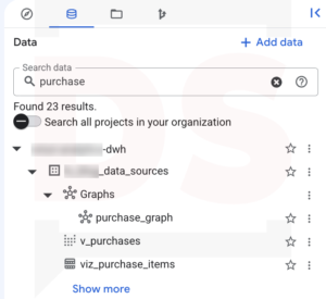
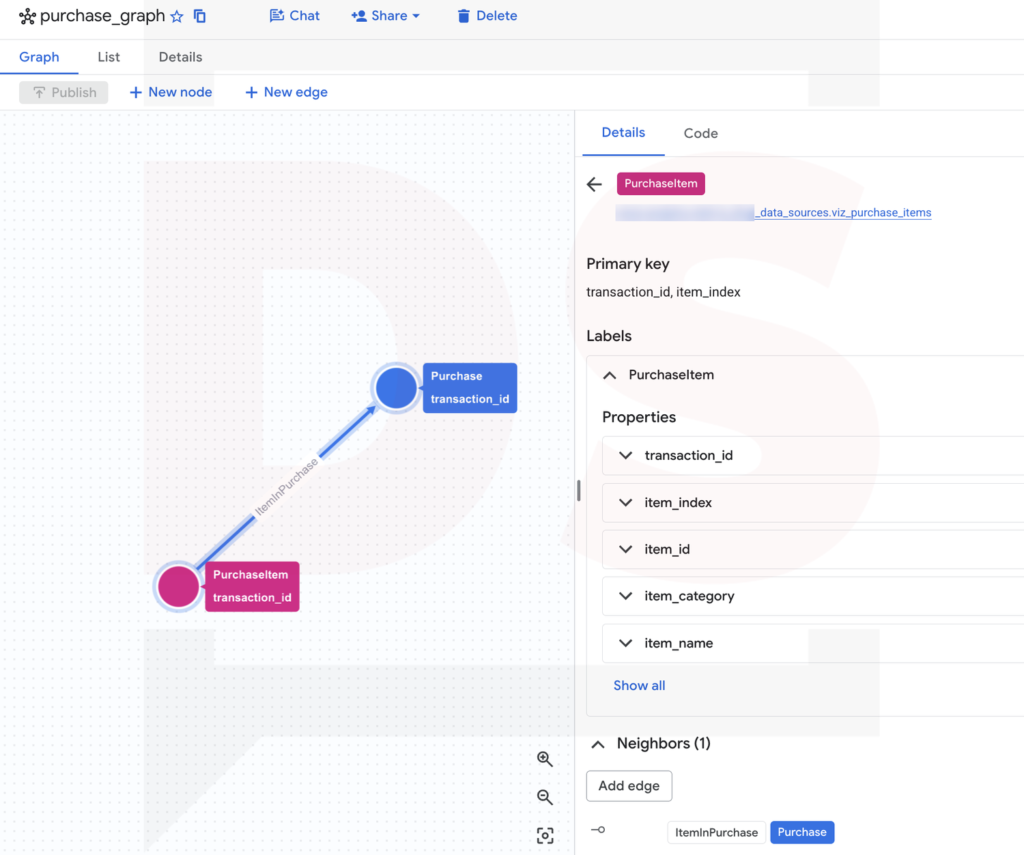
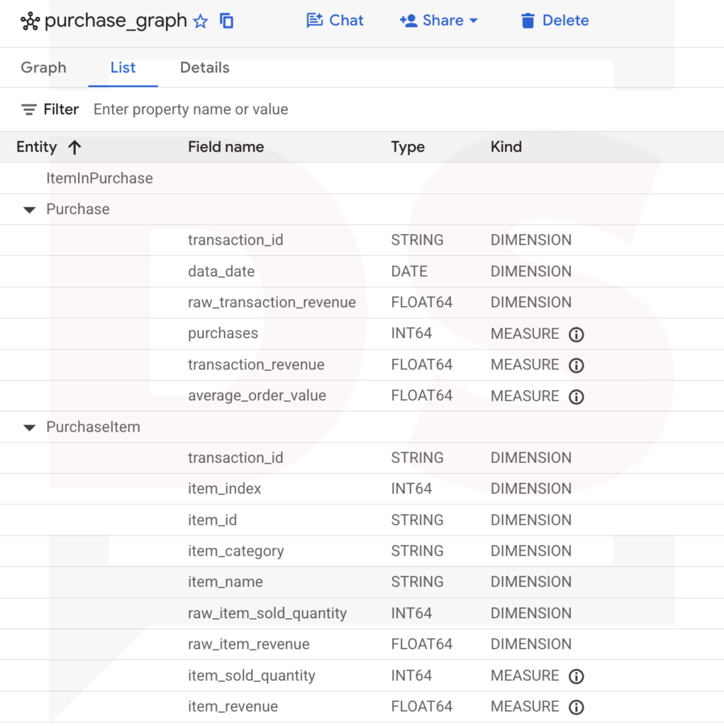
Open the graph from the Explorer to see what the script produced.

• The Graph tab shows the schema: the PurchaseItem and Purchase nodes, linked by the ItemInPurchase edge. Click a node to see its source table, its key and its properties.

---

---

• The List tab lists every property, with a Kind column: DIMENSION or MEASURE. It’s the quickest way to check that your measures are declared.

---

---

Measures check with GRAPH_EXPAND

Before going to Data Studio, if you wish to check the measures with the same business question as the simple query, this time through the graph.

Order and item measures by category

SET @@location = 'EU';

SELECT
  PurchaseItem_item_category AS item_category,
  AGG(Purchase_purchases) AS orders,
  AGG(Purchase_transaction_revenue) AS order_revenue,
  AGG(Purchase_average_order_value) AS average_order_value,
  AGG(PurchaseItem_item_revenue) AS item_revenue
FROM GRAPH_EXPAND("your-project.your_dataset.purchase_graph", start_node => "PurchaseItem")
GROUP BY ALL
ORDER BY order_revenue DESC;

Explanation of the query:

• GRAPH_EXPAND flattens the graph from the item node, with one column per property, named <Node>_<property>.
• AGG() applies each measure at the grain of its node: once per order for Purchase_*, once per item line for PurchaseItem_*.
• SET @@location gives the location of your dataset. The graph is only referenced by a string here, so BigQuery can’t guess it. Replace EU with your own location.

Check that the order_revenue and average_order_value values are consistent with the expected results.

---

The BigQuery Graph as your Data Studio data source

Now, let’s add a data source to the report with the BigQuery connector and the following configuration:

• Project: your project in My Projects, then your dataset.
• Table / Graph: purchase_graph. Graphs have their own icon in the list.
• Start Node: empty. Our graph has a single root, the item node. A start node is only needed when the graph has several.

[Image 6] Data Studio, connecteur BigQuery : liste Table / Graph avec l’icône de graphe, et liste Start Node. Caption: BigQuery Graph selection in the Data Studio BigQuery connector Fichier : 6_bigquery_graph_selection_in_the_data_studio_bigquery_connector.png

In the data source, the graph measures are imported as metrics, in a dedicated Metrics / BigQuery Measures section, and named <Node>_<measure>, like Purchase_transaction_revenue. Their aggregation is displayed as Auto, without any menu to change it: it’s defined by the graph. You can still edit their data type and their description.

---

---

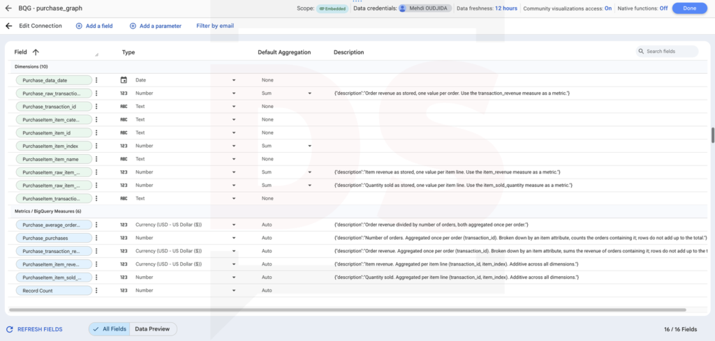
Guardrail: no chart can turn the order revenue measure back into a simple sum. The raw_ fields remain available as dimensions, and their description points to the measure to use.

---

Data Studio charts configuration

At last, let’s create the charts. All of them use the same data source, and none of them needs a blend, a custom query or a calculated field.

---

---

Scorecards for order and item totals

Four scorecards (1), without any dimension:

• Orders: Purchase_purchases.
• Order revenue: Purchase_transaction_revenue.
• Average order value: Purchase_average_order_value.
• Item revenue: PurchaseItem_item_revenue.

Nothing special, and that’s the point: on the flat table, the order revenue scorecard would already be inflated by every multi-product order.

Table chart by product category

A table chart with the configuration below:

• Dimension: PurchaseItem_item_category (2).
• Metrics: Purchase_purchases, Purchase_transaction_revenue, Purchase_average_order_value and PurchaseItem_item_revenue (3).

The order metrics and the item metrics sit side by side in the same row, each one at its own grain.

One rule to keep in mind: the rows don’t add up. An order containing Apparel and Bags counts in both rows, which is right for each category. The sum of the rows is higher than the total revenue, and it should be.

And the grand total (4), on the other hand, is right too!

---

Configuration review

As usual, let’s review the full configuration with this small video.

---

Promising BigQuery Graph

For years, Data Studio users working on BigQuery have handled mixed grains with discipline: one table per grain, blends, custom queries, and a lot of warnings in the report descriptions. Graph measures don’t add a new calculation. They move the aggregation rule where it belongs, next to the data, and Data Studio enforces it.

This tutorial describes only one case. The same pattern applies wherever your reporting tables repeat a value from a higher level:

• Session revenue repeated on each page view, to get the value of the sessions that viewed a page or a content group.
• User attributes and lifetime value repeated on each session, broken down by traffic source or device.
• Campaign costs and conversions recorded at different levels, sharing the same campaign dimension.

And there is a bigger picture. A graph with measures, descriptions and synonyms is a semantic layer that lives in BigQuery. Conversational analytics already relies on it: BigQuery data agents can use the measures of a graph to aggregate at the right level, and these agents can be used from Data Studio. Declaring the grain in the model is far more reliable than explaining it in prompt instructions.

I’m currently exploring this side with BigQuery data agents and Conversational Analytics in Data Studio. But that’s another story.